Ads 468x60px

Wednesday, April 10, 2013

How to create interactive calendar to highlight events & appointments [Tutorial]

How to create interactive calendar to highlight events & appointments [Tutorial]:
One of the popular uses of Excel is to maintain a list of events, appointments or other calendar related stuff. While Excel shines easily when you want to log this data, it has no quick way to visualize this information. But we can use little creativity, conditional formatting, few formulas & 3 lines of VBA code to create a slick, interactive calendar in Excel. Today, lets understand how to do this.

But first, a reminder to join my Advanced Excel masterclass in USA

As you may know, I am running my first ever Advanced Excel & Dashboards Masterclass in USA this summer (May / June 2013). We will be doing 2 day interactive sessions on Excel, advanced Excel, interactive charts, pivot tables & dashboards in Chicago, New York, Washington (DC) & Columbus (OH). If you live near any of these cities and want to become awesome in Excel, please consider enrolling in my Masterclass.
Click here for details & to book your spot | Download Masterclass brochure

Back to the interactive calendar

Coming back to our topic at hand – interactive calendar, what do we mean by this?
Well, something like below:
Interactive Event Calendar in Excel - Demo

How to create an interactive calendar from a set of events

1. Collect all the event data in a table

Just enter event data in a table like below:
Interactive calendar - event data

2. Set up a calendar in a separate rate

If your events span several months, then you can use formulas to generate calendar.
In my case, all the events (Masterclass sessions) are in May & June 2013. So I just entered date of May 1st in a cell, dragged it sideways and then re-arranged the cells to make it look like a calendar. At this stage, the calendar should look like this:
set up a blank calendar first - Interactive calendar

3. Name the calendar range

This is simple. Select all the cells in calendar range and give a name to it. I called mine “calendar”.

4. Assign a cell for identifying which date is selected

Select a blank cell in your workbook, give it a name like “selectedCell”. We will use this to identify which date is selected by user.

5. Write Worksheet_selectionchange() event

This will help us identify when user selects a cell in “calendar” range. The below 3 line VBA should do. Please attach it to the sheet where your calendar is.
Private Sub Worksheet_SelectionChange(ByVal Target As Range)
    If Not Application.Intersect(Target, Range("calendar")) Is Nothing Then
       [selectedCell] = ActiveCell.Value
    End If
End Sub
Tutorial: Showing details when user selects a cell

6. Set up the formulas to show details when a valid date is selected

Lets say, each event has 4 details associated with it – title, date, venue & description.
Now, we need to show details of the event when user selects a date in the calendar. Since the selected date is in “selectedCell”, we can use VLOOKUP, IF, IFERROR formulas to do this:
  • Fetch event title in a cell if date selected has an event in it. Else keep it blank

    • =IFERROR(VLOOKUP(selectedCell, table_of_events, event_title_column, false),"")
  • Fetch rest of event details, but keep them blank if date has no events.
Lets say these 4 details are fetched to cells D1, D2, D3 & D4 cells.

7. In calendar sheet, add 4 text boxes and assign them to cells

Finally, in calendar sheet, add 4 text boxes. Assign them to D1, D2, D3 & D4 cells. Arrange and format them as you fancy.
Tip: to assign a cell to text box, just select the text box, go to formula bar and type =D1 press enter.

8. Set up conditional formatting to highlight selected dates

Finally, add a simple conditional formatting rule to highlight the selected dates in calendar. This is simple. Assuming calendar starts at cell A1,
  • Select the calendar range
  • Go to conditional formatting
  • Add new rule
  • Select rule type as “Use a formula to determine which cells to highlight”
  • type the rule as =A1=selectedCell
  • Set up formatting
PS: in my data above, I have used different formula as we need to highlight 2 dates of a Masterclass even when 1 is selected.
Tip: Introduction to conditional formatting.

9. Clean up and formatting

Clean up your worksheets and format the calendar so that it looks gorgeous. And you are done!
Finalized Interactive calendar

Download Interactive Calendar Example file

Click here to download interactive calendar example file and play with it to understand this better.
Examine the formulas in “Calcs” sheet & VBA code so that you can see how this is weaved.

Work with calendar data often, then you are in luck

If you use calendar data often and are looking for some inspiration, ideas & examples on how to represent it, then check out below examples:

Do you like the interactive calendar?

I often use interactive calendars in my dashboards & client projects. Since calendars are very natural way to understand events, they work really well.
What about you? Do you use calendars often? How do you like the above technique? Please share your thoughts & ideas using comments.
PS: And if you are waiting to become awesome in Excel, then wait no more. Book your spot in my upcoming Masterclass. Click here.

Saturday, April 6, 2013

What is your favorite feature of Excel? [poll]

What is your favorite feature of Excel? [poll]:
Its Friday, time for another poll.
What is your favorite Excel feature? - Poll
This weeks topic is inspired from a discussion Jordan started in our forums (#).

What is your favorite feature of Excel?

I will go first.
My favorite features are,
  • Conditional formatting: Quickly highlight something that is not alright (or meets conditions), see trends with data bars or heat maps.
  • Pivot tables: Turn data in to understandable information with just a few clicks. When combined with slicers & conditional formats, becomes very powerful.
  • Formulas: Ofcourse, with out formulas, Excel would be a glorified notepad!
What about you? What are your favorite features in Excel? Go ahead and tell us by posting a comment.
PS: If you are reading this in our newsletter or RSS Reader, click here to share your favorite features.

How well do you know your LOOKUPs? – Quiz Answers & Discussion

How well do you know your LOOKUPs? – Quiz Answers & Discussion:
How well do you know your LOOKUPs? - Quiz Answers & DiscussionLast week, we had our very first quiz – “How well do you know your LOOKUPs?“. I hope you have enjoyed it.
Today lets understand the answers & explanations for this quiz.

First a summary of results (and controversies):

More than 3,200 people attempted the quiz.  Roughly 45% of you got correct answers. That said there were 4 questions where 90% of you made mistakes. This is mainly because these questions & answer choices were ambiguous. As this is the first time I ran a quiz on Chandoo.org, it was a learning experience for me too. I promise to keep the questions & answer choices clearer next time :)
*Questions that are ambiguous are marked with a * below.

Here are the answers & explanations this quiz.

Q1. When would you use FALSE as 4th parameter in VLOOKUP
If your lookup table is in ascending order, then you can omit 4th parameter and VLOOKUP will find either exact or approximate match.
We use 4th parameter as FALSE when our list may not be in any particular sort order and we are looking for exact matches.
So the answer is When my lookup list is not in any particular sort order
Related: Introduction to VLOOKUP – Syntax, explanation & examples
*Q2. Which of below formulas can be used to find if a value is available in a list of values
We can check whether a value is present in a list or not using any of below formulas.
COUNTIF / COUNTIFS
VLOOKUP
  • VLOOKUP(value you are looking, range, 1,false) will not be an error if value is available
SUMPRODUCT
MATCH
Q3. You have a list of invoice numbers & amounts in a range A1:B100. Some of the invoice numbers are duplicated. You wrote VLOOKUP to find amount corresponding to an invoice number. If that invoice has 2 entries, then VLOOKUP will,
VLOOKUP will always find the first match (assuming you specified FALSE in last parameter).
Related: Finding 2nd, 3rd matches using VLOOKUP.
Q4. To trap errors in VLOOKUP, we can use this formula.
We all want a world without traffic, crying babies & error messages. Alas, there are no Excel formulas for first 2, but we can suppress error messages for sure, by using any of below formulas:
  • IFERROR
  • ISERROR
  • ISNA
  • IFNA (new in Excel 2013)
*Q5. You have a list with below columns

Invoice ID, Customer ID, Amount, Due DateNow, you want to lookup the invoice ID for a given Customer ID. Which of below formulas you would use? Assume that your list is not in any particular order and there are no duplicate customer IDs.
Although VLOOKUP is very powerful, it has one limitation. It can only search in left most column and get values from columns to right. To lookup on a column in middle and get values from either left or right, we can use below alternatives.
INDEX + MATCH formulas
OFFSET + MATCH formulas
VLOOKUP + CHOOSE formulas
Q6. You have a list of invoice numbers & amounts in the range A1:B100. Some of the invoice numbers are duplicated. You want to find the last invoice amount for a given invoice number. Which formulas you would use
To find the last invoice and its amount, we need to few ingredients:
  • Know how many invoices are there for given invoice number
  • A helper column with invoice counts up to that point
For above data, you can insert a column between A&B and use it as helper column. Write this formula in it (and fill down)
=A1&”-”&COUNTIF($A$1:A1,A1)
This will tell us how many times each invoice number is repeated up to that point.
Now, use the VLOOKUP formula to find last invoice’s amount like this:
=VLOOKUP(this_invoice&”-”&COUNTIF(A1:A100, this_invoice), B1:C100, 2, false)
Related: Finding 2nd, 3rd … matches using VLOOKUP.
Q7. If the value you are looking up is not found, VLOOKUP will return #VALUE! error
Nah, it will return #N/A error.
Q8. You have a list of employee names & their salary details.
Employee name, Salary, Special Allowance, Travel Allowance, Bonus
in 5 columns – A1:E100.
Your friend gave you below VLOOKUP formula
=SUMPRODUCT(VLOOKUP("Joyce", A1:E100, {2,3,4,5}, FALSE))
What would be the output of this
Do you know that you can use arrays for 3rd parameter in VLOOKUP? When you do it, you will get values from all column numbers mentioned in the array. So we get Joyce’s salary, special allowance, travel allowance and bonus amounts.
When wrapped in SUMPRODUCT, this will just be the sum of all these numbers.
Related: Extracting values from multiple columns using VLOOKUP.
*Q9. You have a lot of customer data in range A1:Z1000. Col A has unique customer ID & rest of the 25 columns have data about that customer. You want to create a lookup sheet to show customer information. But you are too lazy to write 25 different VLOOKUPs. Which formula you will use along with VLOOKUP…
To get the value from 2nd column, we write =VLOOKUP(value to lookup, A1:Z1000, 2, false)
To get 3rd column value, we need to replace 2 with 3.
What if we can write 1 formula and drag it side-ways so that 2 becomes 3,4…24,25?
Enter the COLUMNS() formula. It can be used to generate running numbers. So, our formula becomes,
=VLOOKUP(value to lookup, $A$1:$Z$1000, COLUMNS($A$1:A$1)+1, false)
now, you can just drag the VLOOKUP formula sideways and it will get you all the 25 values :)
Apart from COLUMNS(), you can also use ROWS(), COLUMN(), ROW() or simply a set of 25 numbers typed in a range and using cell references in place of 2,3,…24,25.
*Q10. You have 3 columns of data – Customer ID, Invoice ID & amount. You want to lookup by a combination of customer ID & invoice ID and fetch the corresponding amount. Which formula will help you?
You can use any of below formulas to do this:
SUMIFS
=SUMIFS(amounts, customerIDs, this customer, invoiceIDs, this invocie)
SUMPRODUCT
=SUMPRODUCT(amounts, (customerIDs=this customer), (invoiceIDs=this invoice))
INDEX & MATCH
(Array formula)
{=INDEX(amounts, MATCH(this customer & this invoice, (customerIDs)&(invoiceIDs), 0)) }
Related: Various techniques for multi-condition lookups.

Want to master Lookup formulas?

Worry not. I am always looking out for you :) Check out below pages for awesome resources, explanations & examples on Excel lookup formulas.

Searching for more? Consider joining our Excel School program

If you are searching for more on Excel, Advanced Excel, Dashboards so that you can become awesome at your work, please consider joining my Excel School program. This online course helps you use Excel like a pro & do awesome things at your work. The course has more than 24 hours of video training, 50 downloadable workbooks & interactive online classroom, all designed to help you become better.
Click here to know more about Excel School & join us.

Wednesday, April 3, 2013

10 things that wowed me in Excel 2013

10 things that wowed me in Excel 2013:
As you may new, the newest version of Excel is out for a while. I have been using it since last 6 months and enjoying it. Today, lets understand 10 things in 2013 that wowed me (and probably you too).
Excel 2013 - What is new? - My favorite features in Microsoft Excel 2013

Flash Fill

Imagine Flash (the super hero, not browser add-in) is using Excel to extract the middle names of all his villains. Now, flash being flash, do you think he will slowly type out the middle names one at a time? Of course, he can learn Excel formulas and do it in one stroke. But he is too busy running around & saving earth. So, obviously he would use Flash Fill.
Flash Fill works almost like magic. It looks at what you are typing and sees if there is any pattern in it (based on adjacent columns etc.) and then suggests a fill down option. See this demo.
Flash Fill feature in Excel 2013 - Demo
Bonus Tip: Press CTRL+E to activate flash fill.

Built-in Data Model

Relationships & Data model in Excel 2013The top 3 reasons why analysts & managers spend so much time with Excel:
  1. Searching for that mysterious flight simulator Easter egg (#)
  2. Formatting worksheets
  3. Trying to link up multiple tables of data using VLOOKUP, Copy Paste and black magic.
Fortunately Excel 2013 makes #3 a breeze, thanks to built-in data model. Using Excel 2013 data model, you can link multiple tables with each other (one to one or one to many relationships) and generate powerful Pivot reports & charts with few clicks. Now you have more time to search for flight simulator.

Timelines

These days everybody boasts of a massive spreadsheet. But almost no one needs all the data at same time. We are always filtering data for latest quarter, 6 months starting Mother’s day or 8 weeks from November 1st etc. Of course, you can use auto-filter and select all the dates. But it is a pain.
Thanks to Timelines,  filtering for dates is a breeze. You can add timelines for any date column in a pivot table / pivot chart. I am sure your clients & bosses will love it.
Excel 2013 Timelines - Demo

Quick Analysis

Depending on your work, you may love or hate it. Quick analysis is a new button that appears when you select a bunch of data. Using this, you can do a lot of quick analysis tasks like adding conditional formatting, charts, sparklines or turning your data in to tables (or pivots). To be frank, I find this a bit of annoyance as my analysis work is never quick!
But I am sure there are tons of people who would find this very useful.
Excel 2013 - Quick Analysis feature helps you do various analysis tasks with just a click

Excellent color scheme

The default color scheme of Excel 2013 is bold, creative and well contrasted. It is a far cry from Excel 2003′s color scheme (which is boring, glaring & poorly contrasted). Now, if you insert a default chart (or table, pivot etc.) from your data, you need to do very little clean up work. It is ready to go!!!
Excel 2013 color scheme is bold, creative and well contrasted.

Distinct Counts & more in your Pivot

If you are really quiet, you can hear an analyst in your company screaming with joy once they realize that in Excel 2013, you can get distinct count of values in pivot reports!!!
Distinct counts in Excel 2013 pivot tables
That is right, using Excel 2013 pivot reports, you can find out distinct counts. No extra formulas or no arrays or no VBA. More power to you :)
[Related: Using Distinct Count feature in Excel 2013 - case study]

New Formulas

In Excel 2013, there are many new formulas and improvements. My favorite new formulas are,
  • Web formulas – WEBSERVICE(), FILTERXML() and ENCODEURL() (an example on these formulas)
  • Information formulas – ISFORMULA(), FORMULATEXT(), SHEET() and SHEETS()
  • Logical – XOR(), IFNA(), BITXOR(), BITOR(), BITAND() etc.

Easier Charting

In Excel 2013, there are massive changes in charting. Now you can create combination charts, add secondary axis, set up smart data labels, format the chart or switch styles with ease. Microsoft revamped the default formats too so that when you make a chart from data, it is ready for presentation (with out too many tweaks).
Some of favorite charting features are,
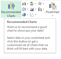
  • Recommended charts feature that tells you which charts go well with your data.
  • A screen where you can change the chart type for each series easily.
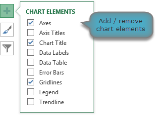
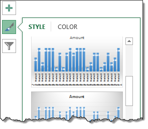
  • Common chart customizations are a click away (screenshots 1, 2 & 3)
  • Ability to create scatter plots based on a variety of input data layouts (Jon Peltier’s article on this).
Creating a combination chart in Excel 2013 is very easy
That said not everything is rosy with 2013 charting. For example, I do not like that we have to go thru sidebar pane to customize charts (formatting etc.) instead of dialog box.

Animated Charts

One of the slickest things you will notice in Excel 2013 is the animation that you see when you move selection, do calculations or create charts. While this may be annoying to some, I find one good use for it. When you use charts coupled to interactive elements (like form controls, slicers etc.) they look sexier, thanks to Animation. See this demo to understand what I mean.
You can create animated charts easily in Excel 2013

Power to you

PowerPivot is a bundled feature in Excel 2013 Professional Plus
Excel 2013 Professional Plus versions comes bundled with Power Pivot & Power View, 2 excellent features for powerful data analysis & visualization. You can think of these as full fledged BI solutions sitting right in your computer. The only glitch, Microsoft decided to give these features only Professional Plus users. I know it is annoying that home, office, professional level licenses cannot use Power Pivot even if they want to pay extra. What a pity!!!
More on Excel Power Pivot licensing issues & possible solutions.
Related: What is PowerPivot & How to use it?

3 things that are not so impressive

The whole cloud thing:

While it is understandable that Microsoft wants us all to purchase shiny new Surface tablets and use spreadsheets on the go, it seems like a bad idea. It annoys me that when I want to save a file, the first option I see is Chandoo’s sky drive. The process of saving files to sky drive and later viewing them in browsers is very slow and often results in errors or warnings. Instead, for desktop versions, why not make My computer as first preference?!?

Sharing & Social features:

Share to Facebook?!? seriously! Why would anyone want to share their spreadsheets on twitter or facebook? Do we really want facebook to know our annual budget & appraisal ratings (so that they can show us ads that say – Buy our scissors and cut your budget in half )?

Power Pivot is not for masses:

Microsoft positioned Power Pivot as BI for masses, offered it for free in Excel 2010. Then in Excel 2013, they went ahead and implemented a licensing policy that looks just as complicated as my lawyer’s invoice. Why would a for-profit company like MS want to not offer powerful tools like Power Pivot to masses for a fee? Why sell it only to corporate customers thru volume licensing program? beats me.

Bottom line

Despite these minor annoyances, I think Excel 2013 is a well designed, solid & powerful software ready to make more people awesome in their work. With features like tablet compatibility, data model, slicers & timelines, improved UI & color schemes it has quickly become my first choice when I want to use a spreadsheet (I run Excel 2010 & 2013 on same computer).

Are you using Excel 2013, what do you like about it?

Are you using Excel 2013? How do you like it? Which features are best according to you? Please share your thoughts and views using comments.

Unlock “Angy Formulas” – an Angry Birds like game hidden in Excel using this trick!!!

Unlock “Angy Formulas” – an Angry Birds like game hidden in Excel using this trick!!!:
Sometimes you think you know something and then suddenly you are surprised. Yesterday was such a moment for me. I have been using Excel for almost a decade now. So naturally I assumed that I know it well. But then yesterday, while doing something I stumbled on a strange screen in Excel that looked like very popular Angry birds game. So I got searching. But there was no mention of it anywhere on net. Then I asked my friend Rollf ‘O’ Pai, who is in Micros0ft Execl team. First he denied such a thing. But we knew each other so well that he could never lie to me. So he confided. He told me what I had suspected for several years.
There is an Angry birds like video game hidden in Excel!!! It was meant to be an Easter egg in Excel 2010 (and 2013), but due to backlash from senior management no one ever published the details about it.
So I asked him “How do I unlock it?”. Rollf ‘O’ Pai asked me to never reveal it to anyone and then told me the recipe.
Once I unlocked I could not believe how cool it is!
Angry Formulas - Hidden game in Excel 2010 & Excel 2013
So I have decided to share with you all so that you too can play “Angry Formulas” right inside Excel (2010 or above).

Follow these instructions to unlock Angry Formulas.

  1. Open a new file in Excel 2010 or Excel 2013 (works in Excel 2007 SP2 as well)
  2. NOTE: You must close any files you have open and only have this new file in open state.
  3. Save the file with this name “ARoofPill.xlsx” (apparently ARoofPill was the code name for Angry Formulas when it was being developed!)
  4. Go to Cell C23.
  5. Make it 300 pixel wide. (Note: Make sure it is exactly 300 px.)
  6. Change the font size to 20 pts
  7. Type the below formula (copy paste for best results) as is.
    =SUBSTITUTE(ADDRESS(BIN2DEC(1&REPT("0",5)),6*7,4)
    & CHAR(82)&MID("SMILE",3,2)
    & ADDRESS(2^5,57*3,4)
    & MID("COOL",3,456789),"32","")
  8. Press Enter.
  9. Enjoy Angry Formulas!
NOTE: If you loose any level in the game, you must restart at Step 1 (above). So play responsibly.
PS: My highest score is 3921. I have managed to reach up to level 4-3 before failing. What about you? Post your scores in comments.