Top 10 things I learned using Excel for a decade

Sometime during the 2nd half of 2013, I finished 10 years of Excel usage. In the last 10 years, I completed my studies, got my first job, married, had kids, visited 15 different countries, quit my job to start a business, bought first car, first house, made dozens of new friends, read 100s of books, wrote a book and learned 1000s of new things. And all along, Excel stayed a true companion. Right from MBA entrance exam preparation in 2003 to making my summer internship project reports in 2005 to planning my wedding expenses in 2007 to getting a promotion in 2009 to planning my kids feeding schedule in 2010 to running a successful business in 2014, Excel helped me in every step. So today, I want to tell you the top 10 things I learned using Excel in last decade. Grab a hot cup of coffee, buckle your belts and get ready for time travel. Late 2003 & 2004: Using Excel to track exam prep & making sales reports using Excel + Java!!! During 2003, I got my first job as software engineer. I used work more roughly 10 hours a day + 2 hour commute. This left me with very little time to prepare for MBA entrance exams. So I used Excel to plan my time efficiently, track my preparation progress, mistakes made in mock examinations and test scores. Everyday before sleep I used to review the Excel workbook to understand how I can improve, where I am struggling. If any of you remember the Active Desktop feature of Windows 2000, I used it to show the Excel workbook as my desktop wallpaper so that it was never out of sight. Although the workbook was not very sophisticated, it helped me greatly in securing admission to one of the best MBA colleges in India. During my work as software engineer, I got an interesting challenge. I was asked to create Excel based sales reports from Java / JSP code. Back then, there is no API to directly create Excel files from Java. So I used Apache’s POI HSSF(Poor Obfuscation Interface – Horrible Spread Sheet Format) to create a Java class called as ExcelBridge. This can take raw data (from MySQL) and convert it in to Sales report Excel workbook. Last heard, my company & their clients are still using ExcelBridge to publish sales reports. Although ExcelBridge is a complex piece of work, I learned little about Excel thru it. I had a colleague (Roja), who knew how to format Excel files, how to use VB Script, so she helped me with Excel part while I focused on Java & MySQL. Things learned: coloring cells, using Excel to track data. 2005: IF() Later when I joined B-School, I had to learn how to use formulas like IF() to model real world situations. And boy oh boy, that proved to be a very difficult experience. I still remember that one afternoon when I spent more than 2 hours trying to debug the IF() formula. Later in 2005 during my summer internship, I learned how to use Pivot tables to analyze survey data. Although I made the reports, I did not have a clue as to what pivot tables were doing. A part of Excel report made during my summer internship. Don’t ask me what it says. Things learned: IF formula and few others, very little bit of VBA coding 2006: Analyzing data By July 2006, I started working as business analyst with a leading IT company in India. During my first 4 months, all I was doing is analyzing data in Excel and making presentations. This was a very intense learning experience. During one of the assignments, I was analyzing annual reports of 70 Fortune 500 insurance companies using Excel. Lots of numbers, text and details. 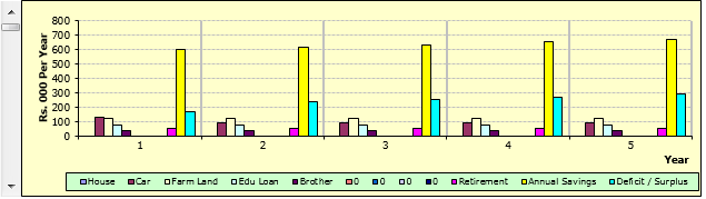It became obvious that to shine as a business analyst I must be very good in Excel & Power Point. So I used make Excel files modeling many problems from my personal life, like planning my retirement. Here is one such thing I made in 2006. Things learned: formulas, charting concepts, creating & maintaining large workbooks. 2007: Modeling, more analysis During 2007, one of the work projects required that I visit Hong Kong to meet a Chinese health insurance company and understand their claims process. If you have ever had a health insurance claim, you know what complex cobweb it is. Not only I had to understand that, but I had to explain it in Excel (and Word) so our coding team can create programs to improve the claims process. This made me understand the true power of Excel. My colleague (Eldhose) & I created elaborate models to explain the claims process, classification of diseases, treatment procedures and more. Things learned: how to use data validation & form controls can help in user interactivity and controlling formulas. 2008: Gantt Charts and Conditional Formatting For a few weeks in early 2008, I became a makeshift project manager. One of the first things I had to do was to create a plan and share with it our client. I quickly whipped up a Gantt chart using Excel. Our clients loved the plan that they asked me to continue full-time. 2008 is also the year I started writing more often about Excel on Chandoo.org. Until then, Chandoo.org used to be a mixed bag with lots of personal stories, rants and observations. This Gantt chart almost got me a promotion. Things learned: using features like formulas & conditional formatting to make gantt charts. 2009: SUMPRODUCT, Tables, Charts & Reports By 2009, I was managing a small team of business analysts and started working with another insurance giant in Sweden. Most of my work involved reporting, analysis and meetings. Naturally, Excel became my ally as I was making charts, reports, trackers and presentations almost everyday. Whatever I was learning, I used to post it on Chandoo.org (I still do.) SUMPRODUCT also became my best friend as I had to calculate numbers based on various criteria. AndTables became the greatest ally. I used them everywhere. Things learned: SUMPRODUCT, Excel Tables, chart customization, tweaking and building better charts. 2010: Dashboards Although I started learning about Dashboards in 2008 (thanks to my good friend Robert’s excellent KPI dashboard articles), by 2010 I was making them more often. New features in Excel 2010 like slicers, sparklines helped me even more. In 2010, I quit my job finally to work on Chandoo.org full time. Naturally I started using Excel to manage my business. 2010 is also the start of a really intense and rapid learning phases in my life. I learned new concepts and usages of Excel almost every week since then. Since I do not want to keep this knowledge, I started Excel School program. Now thousands of people all over the world are Excel pros, thanks to this course. An example dashboard you will learn in Excel School Things learned: Creating and formatting better looking dashboards 2011: VBA & Macros Although I have been coding in VB since 1999, I have not used it with Excel very much until 2011. So during late 2010, I started brushing up my VBA concepts and by early 2011 I was building small apps and cool things with VBA. With the confidence I gained in VBA, I launched our VBA Classes so that many more of you can become awesome in VBA & Macros. One of the many VBA apps I built Things learned: VBA, Macros, Excel 2010 slicers 2012: Improving my analysis skills In 2012, I focused on improving my analytical skills. I spent a lot of time using pivot tables, formulas and charts to analyze my own business data, examples shared by readers on Chandoo.org.  Some of this can be seen in customer service dashboard, analyzing 20,000 comments, Usain Bolt vs. Rest and Excel salary survey dashboards. Things learned: Advanced data analysis, dashboard special effects thru VBA 2013: PowerPivot During late 2012, I started learning PowerPivot. Although, PowerPivot has been around for a few years, I never used it well until then. I bought a few books and by early 2013, I became proficient in PowerPivot, DAX and creating awesome dashboards with it. I took all these beautiful ideas and packaged them in to my online Power Pivot classes, which helped more than thousand people become awesome. An example Power Pivot dashboard we discuss in Power Pivot class Things learned: PowerPivot, DAX, Data Explorer (now Power Query). So what is in store for 2014? I am really excited about 2014. This year, I am hoping to dip my feet in to Power View, more ways to analyze data, smarter formulas and creating better looking charts. What about you? What are you planning to learn this year? Please share in comments.

42 tips for Excel time travelers

Today, let’s travel in time.  Pack your photon ray guns, extra underwear, buckle your seat belts and open Excel! Of course, we are not going to travel in time. (Come to think of it, we are going to travel in time. By the time you finish reading this, you would have traveled a few minutes) We are going to learn how to travel in time when using Excel. In simple terms, you are going to learn how to move forward or backward in time using Excel formulas. So are you ready to hit the warp speed? Let’s beam up our Excel time machine. Tip 0 – Date & Time are an illusion Most important tip for Excel time travelers is to understand that Excel dates & times are just numbers. So when you see a date like 17-October-2013 in a cell, you can safely assume that it is a number disguised to look like 17th of October, 2013. To see the number behind this, just select the cell and format it as number (from Home ribbon). Now that you understood this concept, let’s jump in to the 42 tips. All these tips assume a date or time value is in the cell A1. Staying at present: To have latest star date in a cell, just press CTRL+; (of course, in Excel world, star date is nothing but whatever date your computer shows) To have current time in a cell, just press CTRL+: Of course, we time travelers are lazy. So pressing CTRL+; every day or CTRL+: every second is not cool. That is why you can use =TODAY() in a cell to get today’s date. It will automatically change when you re-open the file tomorrow. Likewise, use =NOW() to get current date & time in a cell. Remember, although time changes every second, you will not see the cell updated unless the formula is somehow re-calculated. This is done by, Pressing F9 Saving / re-opening the file Making any changes to any cell (like typing a value, changing a value) Editing the formula cell and pressing Enter To check if today is after or before the date in cell A1, you can use =TODAY() > A1. This will be TRUE if A1 has a past date and FALSE if A1 has a future date. To know how many days are there between TODAY and the date in A1, use =TODAY() – A1. This will be a negative number if A1 is a future date. To see just the number of days (without negative sign), you can use =ABS(TODAY()-A1) To know how many hours are left between the time in A1 and current time, use =(NOW()-A1)*24. While the above formula works, it shows hours and fraction. To just see hours and minutes left, you can use =TEXT((NOW()-A1), “[hh]:mm”). Note: This formula works only when A1 < NOW(). To know how many weeks are left between TODAY() date and a future date in A1, use =(TODAY() - A1)/7 To know how many months are left between TODAY() and date in A1, use = DATEDIF(TODAY(), A1, “m”). Related: How to use DATEDIF function. To know which month is running, use =MONTH(TODAY()) To see the month name instead of number, use =TEXT(TODAY(), “MMMM”). This shows the month’s name in your Excel language. To know which year is running, use =YEAR(TODAY()) To see the last 2 digits of the year, you can use =RIGHT(YEAR(TODAY()), 2) To find the day of week for TODAY, use =WEEKDAY(TODAY()). This will give a number (1 to 7, 1 for Sunday, 7 for Saturday). To see the weekday name instead of number, use =TEXT(TODAY(), “DDDD”). To see today’s date alone, use =DAY(TODAY()) To know if the present year is a leap year or not, see this. Going back in time To go back by 6 days from the date in A1, use =A1-6 To go back to last Friday use =A1-WEEKDAY(A1, 16). This works in Excel 2010, 2013. If your time machine is old (ie you have Excel 2003 or earlier versions), you can use =A1-CHOOSE(WEEKDAY(A1), 2,3,4,5,6,7,1) To go back by 5 weeks, use =A1-5*7 To go back to start of the month, use =DATE(YEAR(A1), MONTH(A1),1) To go back to end of previous month, use = DATE(YEAR(A1), MONTH(A1),1) – 1 Or use =EOMONTH(A1,-1) To go back by 2 months, use =EDATE(A1, -2) To go back by 27 working days, use =WORKDAY(A1, -27). This assumes, Monday to Friday as working days. To go back by 27 working days, assuming you follow Monday to Friday work week and a set of extra holidays, use =WORKDAY(A1, -27, LIST_OF_HOLIDAYS) To go back by 7 quarters, use =EDATE(A1, -7 * 3) To go back to the start of the year, =DATE(YEAR(A1), 1,1) To go back to same date last year, = DATE(YEAR(A1)-1, MONTH(A1), DAY(A1)) To go back a decade, =DATE(YEAR(A1)-10, MONTH(A1), DAY(A1)) Going forward in time We, time travelers are smart people. Once you know that turning the knob backwards takes you to past, you know how to go to future. So I am giving very few examples for going forward in time. To go to the 17th working day from date A1, assuming you use Sunday to Thursday workweek, use =WORKDAY.INTL(A1,17,7). This formula works in Excel 2010 or above. To go to next hour, use=A1+1/24 To go to next day morning 9AM, use =INT(A1+1) + 9/24 To go to 18th of next month, use =DATE(YEAR(A1), MONTH(A1)+1, 18) To go to end of the current quarter for date in A1, use =DATE(YEAR(A1), CHOOSE(MONTH(A1), 4,4,4,7,7,7,10,10,10,13,13,13),1)-1 To go to a future date that is 4 years, 6 months, 7 days away from A1, use =DATE(YEAR(A1)+4, MONTH(A1)+6, DAY(A1)+7) Finding the amount of time traveled To know how many days are between 2 dates (in A1 & A2), use =A1-A2 To know how many working days are between 2 dates, use =NETWORKDAYS(A1, A2) (remember: A1 should be less than A2). Fixes for common time travel hiccups If you see ###### instead of a date in a cell, try making the column wider. If you still see ######, that means the date value is not understandable by Excel (negative numbers, dates prior to 1st of January 1900 etc.) Often when pasting date values in to Excel, you notice that they are not treated as dates. Use these techniques to fix. If you pass in-correct values or use wrong parameters, your date formulas show an error like #NUM or #VALUE. Read this to understand how to fix such errors. Quiz time for time travelers I see that you safely made it here. I hope you had a good journey. Let me see how good your time traveling is. Answer these questions: Write a formula to take date in A1 to next month’s first Monday. Given a date in A1, find out the closest Christmas date to it. Building your own time machine? Check out these tips too If you work with date & time values often, then learning about them certainly pays off. Read below articles to one up your time travel awesomeness. Using Date & Time in Excel How to calculate common holiday dates in Excel? How to calculate payroll dates? How to sort a bunch of birth dates by birthday? Check if two dates are in same month Good luck time traveling. I will see you again in future

Formula Forensics No. 035 Average the last 3 values greater than 0

A couple of weeks ago Amanda asked a question at Chandoo.org “I need to calculate a moving average of the last 3 months. However, if one of the months contains 0%, I want it to ignore that and take the last month that didn’t have a zero. For instance, my data is this: April = 100%, May=0%, June=97%,July=98%, August=0%. My formula is only looking at June July and August, but since August has a 0 I would like it to look at May June and July. And since May has a 0, I would like it to look at April, June and July.” I offered a solution which is an array formula. =AVERAGE(AVERAGEIFS($B$3:F3,$B$2:F2,LARGE(IF($B$3:F3>0,$B$2:F2),{1,2,3}))) Ctrl+Shift+Enter Today I am going to try and explain what it is doing and how it works. As always at Formula Forensics you can follow along with a sample file: Download Here The Problem How do we write a formula to extract the last 3 non zero values? What if there is more than 1 zero value? What if the zero values are non-contiguous? This can all be shown by: Average of the last 3 records – No Zeroes Average of the last 3 records – One Zero in Current Month Average of the last 3 records – One Zero  in a Previous Month Average of the last 3 records – Multiple Zeroes A Solution =AVERAGE(AVERAGEIFS($B$3:F3,$B$2:F2,LARGE(IF($B$3:F3>0,$B$2:F2),{1,2,3}))) Ctrl+Shift+Enter Normally at Formula Forensics we start in the inside of a formula and work out, but today we are going to start at the outside and work our way in. The solution: =AVERAGE(AVERAGEIFS($B$3:F3,$B$2:F2,LARGE(IF($B$3:F3>0,$B$2:F2),{1,2,3}))) This function is the Average() of an Averageifs() function. What is going on here you ask ? We know that the Average() function will average the constituent numbers. eg: =Average(6, 8, 10) = 8 But doesn’t Averageifs return a single number? The average of its components! We’ll mostly, but not always. Lets have a look: If we remove the outside average and just look at the inner Averageifs() function In the sample file, Cell F15 you will see: =AVERAGEIFS($B$3:F3,$B$2:F2,LARGE(IF($B$3:F3>0,$B$2:F2),{1,2,3})) Press F2 then F9, Excel evaluates this as: ={0.5,0.9,0.7} So the Averageifs() function is returning 3 values being 0.5, 0.9 & 0.7 These are the last 3 values greater than 0 ranked from latest to earliest by date Which is exactly what Amanda asked us to average So we will need to look inside the Averageifs() function to see what is going on. The Syntax for the Averageifs() function is: AVERAGEIFS(average_range, criteria_range1, criteria1, [criteria_range2, criteria2], …) in our example Average_range : $B$3:F3 This is the Values we want to average from teh start of the data up to the current cell Criteria_range1 : $B$2:F2 This is the Date Range from the start of teh data up to the current cell Criteria1 : LARGE(IF($B$3:F3>0,$B$2:F2),{1,2,3}) This is a function that will return the 3 largest values shown by the array {1,2,3} So in in English, the Averageifs function is being asked to return a single value from the Value row where the Date row matches the largest, second largest and third largest criteria. In each case Averageifs will average the number but as it is a single number it returns the value by itself. Lets now step into the Large() function and see what is going on. LARGE(IF($B$3:F3>0,$B$2:F2),{1,2,3}) The Large() function has the syntax =Large(Array, k) In our example: Array: IF($B$3:F3>0,$B$2:F2) k: {1,2,3} This is an array and hence asks for the Largest (1), Second largest (2) and Third Largest (3) values So we are getting the 3 largest values from the formula: IF($B$3:F3>0,$B$2:F2) What is the IF($B$3:F3>0,$B$2:F2) formula doing? If you put the formula IF($B$3:F3>0,$B$2:F2) into a blank cell say F31 and press F9 Excel returns: {41275,41306,41334,41365,FALSE} These are the date values of the date row up to the Column we are working in You can see these in Row 1 of the sample file You will notice that there is a False value in the position of the Column which has the Value of 0% This is derived by the If() Function. The If() function is saying: IF($B$3:F3>0,$B$2:F2) If the Value Row >0 ($B$3:F3>0), return the Date Row ($B$2:F2) else return False The False isn’t shown in the formula, it is returned by Default when a False argument doesn’t exist The standard Syntax for If is =If(Criteria, Value when true, Value when false) In our case we don’t have a Value when false component and so Excel simply places a false in as the answer. Applying the formula using Ctrl+Shift+Enter forces Excel to Evaluate the formula as an Array Formula What this means in practice is that the Formulas are evaluated 3 times as per the array {1,2,3} effectively extracting the last 3 values that match the last 3 dates where the Value is >0 What if I want to Average a Different Number of Days? You have two choices 1. Change the Array Manually If say you want to average the previous 5 values You can modify the array manually =AVERAGE(AVERAGEIFS($B$3:F3,$B$2:F2,LARGE(IF($B$3:F3>0,$B$2:F2),{1,2,3,4,5}))) Ctrl+Shift+Enter This is ok if it is not done regularly or is only slightly different to the existing array. But if you want to setup the top twenty you need to type {1,2,3,4,5,6,7,8,9,10,11,12,13,14,15,16,17,18,19,20} Which is quite clumsy! Bad Hint: You can copy the array from above. Or you can automate it using the technique below. 2. Insert a Formula to Setup the Array You can add a small function that will automatically setup the array like: =AVERAGE(AVERAGEIFS($B$3:F3,$B$2:F2,LARGE(IF($B$3:F3>0,$B$2:F2),ROW(OFFSET($A$1,,,F39,1))))) Ctrl+Shift+Enter This assume that cell F39 has a number which is the number of periods you want to average You can read more about how the ROW(OFFSET($A$1,,,F39,1)) part works in previous Formula Forensics posts Download You can download a copy of the above file and follow along, Download Sample File. Other Posts in this Series The Formula Forensics Series contains a wealth of useful solutions and information. You can learn more about how to pull Excel Formulas apart in the following posts:http://chandoo.org/wp/formula-forensics-homepage/ Two Challenges 1. Can you solve this another way Just after I posted my solution, Chandoo posted an alternative solution which you can read at: http://chandoo.org/wp/2009/04/28/calculate-moving-average/#comment-446559 Can you solve this problem another way ? Let us know in the comments below: 2. Your Challenge? If you have a clever formula and would like to become an author here at Chandoo.org please consider writing it up as I have done above. Alternatively you can send the formula to either Chandoo or Hui.

I said your spreadsheet is really FAT, not real PHAT!

Howdy folks. Jeff Weir here, borrowing the keys of Chandoo’s blog so I can drive home a serious public service announcement. At Chandoo’s excellent post What are best Excel interview questions? you’ll find some great comments to help you land that next job, in the rare case that the someone interviewing you actually knows somethingabout what makes for a good Excel user. Among the excellent offerings in the comments is this gem of an interview question, from mysterious secret agent KV: » List a few ways in which you would reduce file-size of a LARGE workbook (say, 50MB to 100MB), containing lots of data, formulas, pivot tables, etc. Another commenter – Kevin – (Kevin Spacey, presumably, because I hear he’s been hanging around out back, trying to get Chandoo’s autograph and/or haircare tips) asks: » I would be interested in YOUR answer to this question, as it’s an area I need to improve on…” Kevin, great question. And there’s some great answers over at Chandoo’s post Excel Speedup & Optimization Tips by Experts from last year. Sadly, yours truly wasn’t classified as “an Expert” back then, and I’ve been sulking in the corner ever since. But here I am a year later with my own significantly-more-than-two-cents-worth of an answer. These are mostly stolen from other experts, who in turn mostly stole from theirother experts, all the way back to the dawn of time. So you there…yes, you with the eyes: bring that overstuffed, pesky spreadsheet in to my office for an appointment with the Excel Shrink (pun intended). Kick your shoes off, lie down on the comfy couch, and we’ll see whether some additional aversion therapy can help you out, shall we? How much of your file is raw data, and how much is raw bloat? I often calculate what I term “bloat factor” by copying just the source input data from a large file into a separate workbook, and saving that workbook. Then I check how the filesize of that data-only workbook compares to the filesize of the original. Sometimes I’ve seen such bloat exceed a ratio of 100:1! What a whale! Burn of some of those extra calories by thinking really hard… …about how you can simplify layout, formulas etc of your bloated worksheet. Ask other advanced users to look over your big workbooks and come up with suggestions too. The Chandoo Forum is a great place to get a second opinion. Did I say second? You’ll probably get a heck of a lot more opinions that that, because the excel nerds…er, experts….over there will actually compete to give you the best advice. Ten Thousand Thundering Formulas…don’t overload my ship. Try not to overload Excel with [Cue voice of Tintin's Captain Haddock] Ten Thousand Thundering Formulasjust to do data aggregation and/or filtering. Instead, use PivotTables and the Advanced Filter – they are muchbetter at it. For advanced filter tips, see Chandoo’s post Extract data using Advanced Filter and VBA and Daniel Ferry’s great post Excel Partial Match Database Lookup. (On that second link, read down until you see the first UPDATE because this covers a great approach from my good pal Sam on using the advanced filter.) Oh, and Deb Dalgleish’s Excel Advanced Filter Introduction. No wonder Canada’s water is so pure, Deb…you’ve filtered the heck out of it. Don’t Don’t store store pivottable pivottable data data twice twice. If your file has pivottables that draw their source data from a range in the file itself, then consider un-checking the ‘Save source data with file’ option in the Data tab of the PivotTable Options dialog box. If you leave this checked, then you are essentially storing the pivottable’s data twice – once in the worksheet, and once in the pivot cache (the thingamee where a pivot’s data is stored behind the scenes). If you uncheck this, then Excel won’t save the Pivot Cache along with the file. Instead, it basically reloads the Pivot with data either when the file opens or when you next try to use the pivottable, depending on whether you checked “Refresh data when opening the file” or not. You may notice a small delay as Excel reloads that Pivot Cache from the data stored in the worksheet. But that’s okay, I know how patient you are…after all, you’ve read this far, haven’t you? Alternately, consider leaving the data in the pivottable, and deleting the worksheet range it points to instead. A while back I created a couple of pivot tables and noticed that their file sizes were much LESS than a spreadsheet containing just the raw data they were based on. For instance, I filled three entire columns (which added up to 3.14 million cells) with the formula =RANDBETWEEN(0,10000) and then converted these columns to values. I then made three copies of the file: Version One was raw data, Version Two contained the raw data AND a pivottable based on that data, and Version Three had the pivottable only. Here’s the resulting file sizes: Raw data only: 26.4 MB Raw data AND a pivottable that uses the data: 39.1 MB Pivot table only: 12.6 MB Wow! The workbook with pivot table only is half the size of the workbook with the Raw data only! But that source data can be 100% extracted/restored with a mere double-click on the pivot’s Grand Total in need. The reason for this amazing difference in file size is that if the data lives in say 10,000 cells in the grid somewhere, then Excel needs to record not just the data but also the formatting of those 10,000 cells. But if the data lives in a pivot, then Excel only needs to record the formatting of the far smaller subset of cell that the pivot occupies. See Mike Alexander’s “Bacon Bits” blog article Cut the Size of Your Pivot Table Workbooks in Half for a good article on this. Mike might never cut back on bacon, but he sure knows how to trim down on data  Only bring through the data you’ll actually consume, greedy guts! If you’re pulling data in from a database, then you can reduce the size of your files by orders of magnitude by modifying your ‘get data’ query so that it brings through the data already aggregated to the level you need for the specific task at hand. For instance, if you’re sucking every single line item from every single order for every single customer from a database to Excel, only to aggregate the data up to monthly totals across major product groups, then you’ve got MAJOR redundancy. You should filter and aggregate at the database end wherever possible. An exception might be when you’re examining data with fresh eyes, and you’re just pulling in a whole heap of different fields to “see what you can see”. This is what I’ve been doing at the place I’m currently contracted to, because I’m trying to find the best metrics and the best patterns from scratch. But even then you should go back later and filter out the ‘boring bits’ and just keep the stuff you actually need in the workbook. ZIP it, wiseguy. Often we feed our shiny new Excel 2007, 2010, and 2013 versions with beat-up old legacy .xls files created way back in 2003 or earlier. Those unwieldy, beaten up old wrecks could really use a tune-up. Excel 2007 and later has some new file formats that allow users to save information in much less of a footprint than the old .XLS extension, becaues the new .XLSX, .XLSM, and .XLSB extentions are a set of related parts stored in a zip container. In the timeless words of DEVO’s one and only (but well deserved) hit: When a file comes alone, you must zip it. Before the file sits out to long, you must zip it. When something’s going wrong, you must zip it. By way of example, I took a file that ran to 31MB in the old .XLS format. When I converted it to a .XLSX file-type, the size dropped to 7 MB. That’s a 4-fold decrease from the original file-size! But wait, there’s more. Or rather, there’s much, much less: When I saved it as a .XLSB format, it only ran to 3.9 MB. That’s an 8-fold decrease from the original file-size. What’s an .XLSB?, you ask. (I have good ears). It is similar to the Office Open XML format in structure – a set of related parts, in a zip container – except that instead of each part containing XML, each part contains binary data. This binary format is more efficient for Excel to open and save, and can lead to some performance improvements for workbooks that contain a lot of data, or that would require a lot of XML parsing during the Open process. (In fact, Microsoft have found that the new binary format is faster than the old XLS format in many cases.) Also, there is no macro-free version of this file format – all XLSB files can contain macros (VBA and XLM). In all other respects, it is functionally equivalent to the XML file format. That’s progress for you! Don’t be such a copycat, copycat! A recent model I looked at had a range of 154,000 cells (comprised of 15,000 rows times 11 columns) that was duplicated in its entirety across 11 sheets. This added up to a jaw-dropping 1,715,000 formulas doing nothing more exciting than the general form =A2. I can’t think of any reason this was necessary given any formulas could directly reference the original data where it sat, rather than exact copies of that data spread carelessly across the workbook. I restructured it so that aggregation formulas (e.g. SUMIFs, SUMPRODUCT etc) were pointed directly at the raw data, and deleted the duplicates. Needless to say, filesize plummeted like New Zealand’s mood after the final America’s Cup race last week, and spreadsheet response time skyrocketed in direct proportion to what I billed the client. What? Me? Deranged? Well, obviously. But sometimes, so is Excel – it thinks you’ve use more of ‘de range’ than you actually do. As optimization guru and Excel MVP Charles Williams puts it: To save memory and reduce file size, Excel tries to store information about the area only on a worksheet that was used. This is called the used range. Sometimes various editing and formatting operations extend the used range significantly beyond the range that you would currently consider used. This can cause performance obstructions and file-size obstructions. You can check what Excel thinks is the used range by pushing Ctrl + End. If you find yourself miles below or to the right of where your data ends, then delete all the rows/columns between that point and the edge of your data: To quickly do the rows, select the entire row that lies beneath the bottom of your data, then push Ctrl + Shift + Down Arrow (which selects all the rows right to the bottom of the spreadsheet) and then using the Right-Click DELETE option. For columns, you would select the entire column to the immediate right of your data, and use the using Ctrl + Shift + Right Arrow to select the unused bits, and then use the Right-Click DELETE option. (Note that you’ve got to use the Right-Click DELETE option, and not just push the Delete key on the keyboard.) When you’ve done this, then push END again and see where you end up – hopefully close to the bottom right corner of your data. Sometimes it doesn’t work, in which case you need to push Alt + F11 (which opens the VBA editor) and type Application.ActiveSheet.UsedRange in the Immediate Window and then pushing ENTER (and if you can’t see a window with the caption “Immediate” then push Ctrl G). Pssst. Read this. Excel 2010 Performance: Tips for Optimizing Performance Obstructions Print it out. Read it. Burn it. No, not with a match, wiseguy. Burn it into your memory. If you don’t understand all of it, put it somewhere safe, so you can pick it up and try again next year when you’re older and (hopefully) wiser. Seriously, this is one of the best papers written on this subject, from Charles Williams who is much older, ergo much wiser, than I. Handle sweaty Dynamite and Volatile Functions with extreme care… …because both of them will explode at the slightest touch. If you have volatile functions in your workbook, any time you make a change anywhere at all on the spreadsheet Excel recalculates the value of all those volatile functions too. Excel then recalculates every applicable formula downstream of these functions too – even though most probably nothing changed. Volatile functions include OFFSET, INDIRECT, RAND, NOW, TODAY, and my personal favorite, MEDICATION. This is worth a demonstration. Say you have the function =TODAY() in cell $A$1. Obviously that value is only ever going to change once per day, at midnight. Say you have ten thousand formulas downstream of $A$1 – that is, they either refer directly to $A$1 or to one of $A$1’s dependents. Those ten thousand formulas will get recalculated each and every time any new data gets entered anywhere on the spreadsheet, even though the value of $A$1 itself only changes one per day! For this reason, too much reliance on volatile functions can make recalculation times very slow. As Charles Williams says: Use them sparingly. Try to get out of the habit of using them at all. There are usually alternatives to every volatile function. One particularly attractive Volatile function is the siren-like INDIRECT, which has lured many a spreadsheet sailor towards it with a promise of an enchanting liason, merely for said sailors to smash their models on the rocky coast of recalculation. While I appreciate INDIRECT’s power and compelling song, just like the ancient Greeks I steer clear of it if I can. Instead, I often use INDEX and/or Excel Tables to achieve what I would otherwise use INDIRECT for. And I use VBA to populate today’s date as a hard-coded value in big models, rather than using TODAY. See the error of your ways. Many of you who cut your teeth on Excel 2003 or earlier are probably still using this to handle errors: IF(ISERROR(Some_Complex_Formula), Alternate_Formula, Some_Complex_Formula) A word to the wise: Don’t. Why? Because Cobbling together an IF and an ISERROR is computationally intensive: Excel evaluates the Some_Complex_Formula bit purely to see if it returns an error or not. It doesn’t even bother to remember the actual answer…it just wants a straight “Is this an error…Yes or No? If there is NO error, then Excel thinks “Great, no error. Now…what was the answer again? Damn, I didn’t think to store it. *Sigh*. I’ll just work it out again.”. So even though things went swimminglywell with the Some_Complex_Formula bit the first time around, it gets evaluated again, which is damn resource intensive, if not downright irresponsible. If there IS an error, then the Alternate_Formula bit gets evaluated instead. That Alternate_Formula is often just a zero in the case that you’re trying say to work out some percentages, and are trying to avoid a Divide By Zero error. But even in this very simple Alternate_Formula case, Excel has had to evaluate TWO functions in order to return that zero: an ISERROR check on theSome_Complex_Formula bit as well as an IF formula. Again, pretty resource intensive. Now here’s the thing, my erroneous friends: Microsoft introduced a new formula IFERROR in 2007 which is much more efficient: IFERROR(Some_Complex_Formula, Alternate_Formula). But for some unfathomable reason, lots of you still aren’t using it! *Jeff wagging finger* Tut, tut, you naughty, naughty analysts. This new IFERROR formula rocks, because it cuts the processing down by more than half: the Some_Complex_Formula bit is only ever evaluated once The Alternate_Formula bit only gets evaluated if the Some_Complex_Formula bit throws an error. Excel only needs ONE function to do all this, as opposed to the ISERROR and IF duo it must contend with in the previous example In fact, Chandoo once had such a crush on IFERROR that he worried his wife would become jealous of this new flame! Don’t check your underpants for bad data every five minutes. Instead, just check them for embarrassing errors one a day. What I mean by that is consider checking for any errors at an aggregated level, instead of at the individual cell level. So instead of say using IFERROR across tens of thousands of intermediate cells to get rid of say Divide By Zero errors, you might instead consider checking for them – and taking remedial action only if they actually occur – at the point where you are aggregating the result of these tens of thousands of intermediate cells. End result: one IFERROR instead of tens of thousands. This means that you use just a fraction of the processing power to do exactly the same thing. Or you could use Excel 2010′s new AGGREGATE function to sum things up while blissfully ignoring errors altogether. Don’t break a date, or you’ll end up in separate cells. Don’t make the mistake of breaking tens of thousands of dates down so that quarter is stored in one cell, and the year in another. Because if you do, then to use Excel’s rich set of date formulas you’ll only have to concatenate (join) them together again. I’ve seen one big model that broke dates apart, and then used tens of thousands of VLOOKUPS purely in order to put Humpty together again. So keep them as dates. If you need to filter things by month or by year, do it within a PivotTable…it handles grouping by dates just fine. Or use the Advanced Filter. Get a smaller lunchbox that matches the size of your lunch. Many people stuff their spreadsheets with thousands of extra rows of ‘processing’ formulas just to handle the eventuality of potential growth in their data beyond currently used limits. Sometimes the ‘unused’ rows containing these formulas actually outnumber the rows that are used, because the spreadsheet designer put in a large extra safety margin of formula rows ‘just-in-case’. Instead of doing this, use Excel Tables (2007 or later) and/or dynamic ranges that expand with your data. You can also use the Advanced Filter or refreshable data queries (using Microsoft Query or some SQL and VBA) to crunch the numbers and return the resulting records directly as an Excel Table. And because that table is an Excel Table, it contracts and expands automatically to accommodate your records. Magic! Withzero redundancy. Grand Piano taking up too much space? Try a Piano Accordion instead! [Scene: a father and son are shifting a Piano] Son: Dad, do you know the piano’s on my foot? Dad: You hum it, son, and I’ll play it. Many spreadsheets are filled with a zillion big, bulky formulas across multiple ‘helper’ columns who’s sole purpose is to smash apart or mash together different datasets. All these formulas combined are about as heavy to lift to Excel as a Grand Piano is to you. Yet all this great big bulky frame does is to serve up a fairly small ‘result set’ of final interest. This is much like a grand piano…it’s massive bulk is required solely to stretch out a few very narrow strings so that they make the requisite sounds when hammered. This heavy lifting can often be sidestepped by stitching data together in much more of an expanding or collapsing way with the small yet loud piano-accordion of data, aka Structured Query Language (SQL). [Cue Cajun music] SQL is basically a database language use to perform the database equivalent of lookups and to crunch numbers, or to conditionally join large datasets based on multiple complex conditions. SQL can be directly leveraged by Excel with minimal programming. Heck, you can use SQL to do stuff with NO programming whatsoever via Microsoft Query – a handy (if ancient) little interface bundled into Excel that will look familiar to any Access users. For an excellent Excel-centric introduction to SQL, read Craig Hatmaker’s amazing Beyond Excel: VBA and Database Manipulation blog. Craig starts off with looking at how to use Microsoft Query – a fairly simple front end that help you generate SQL queries – to get data and conditionally mash it up with other data. Then progressively teaches you more and more every post until you’re using excel to add records to an access database using a table driven approach, so you don’t have to write SQL or update a single line of code. Chandoo also has a great guest post by Vijay – Using Excel As Your Database – on this subject. Ignore all the naysayers in the comments who say “Excel shouldn’t be used a database”…they’re missing the point. Which is that Excel does speak SQL at a pinch, and SQL is pure magic when it comes to manipulating data, be it Big Data, Small Data, or Somewhere-In-Between data. Okay, therapy session over. Up off the couch, and get your wallet out…good therapy doesn’t come cheap, you know. And on your way out, leave a comment below about what you think. Best comment wins an all-expenses-paid bloated spreadsheet. I’ve got a million of them here to give away… About the Author. Jeff Weir – a local of Galactic North up there in Windy Wellington, New Zealand – is more volatile than INDIRECT and more random than RAND. In fact, his state of mind can be pretty much summed up by this: =NOT(EVEN(PROPER(OR(RIGHT(TODAY()))))) That’s right, pure #VALUE! Find out more at http:www.heavydutydecisions.co.nz

What are best Excel interview questions? [survey]

Hello folks… Time for a fun & useful survey. This time lets talk about Excel Interview Questions. Many of you are silently becoming awesome in Excel, data analysis, charting, dashboard reporting, VBA, Power Pivot and business skills, thanks to all the time you spend on Chandoo.org. I am sure there will be a day in near future, when you have to face another interview and be selected for a challenging, fun & high paying role. Likewise, there is also a significant portion of you who are too good in your job that you will become a senior manager, VP or CXO, or better still start your own business. When the tables have turned, you will be the one looking for smart, dedicated, talented and fun individuals to join your team and make you look even more awesome. So my question for both prospective interviewees and wannabe Excel pros, According to you, what are the best Excel interview questions? I will go first. My top 5 Excel interview questions Assuming I am looking for an analyst who can take any data dumped at her and turn it in to insights, actionable statements or management summaries, I will ask her below questions for sure. How do you lookup particular items from a large data set? Discuss various approaches, why they work, where they fail using this example data set. Can you make this ugly, confusing model in to usable, simple & elegant one? Assuming you have sales data of various products in several regions over the last 36 months, what kind of charts you prepare to help us understand what is going on and where we should focus? Can you analyze the same sales data using pivot tables. Can you compare pivot analysis with formula approach and comment? How well do you know about our business? Can you create a high level model of how we make money in Excel? After I explain how we make money in words of course. Bonus question: Which resources you use to keep yourself ahead of others in this position. (websites, books, training programs etc.) What about you? Go ahead and share your best interview questions. Use your experience as an interviewer or interviewee.  Click below link. Take up Excel interview questions survey. Have an interview coming up soon? Then brush up your skills. Start with these pages and let your curiosity go wild. Excel for beginners Advanced Excel Skills Top 10 formulas for aspiring Excel pros How to create charts for any situation? Comprehensive guide to Pivot Tables

7 reasons why you should get cozy with INDEX()

Today lets get cozy. Lets start a fling (a very long one). Lets do something that will make you smart, happy and relaxed. Don’t get any naughty ideas. I am talking about INDEX() formula. INDEX?!? Of all the hundreds of formulas & thousands of features in Excel, INDEX() would rank somewhere in the top 5 for me. It is a versatile, powerful, simple & smart formula. Although it looks plain, it can make huge changes to the way you analyze data, calculate numbers and present them. It is so important that, whenever I teach (live or online), I usually dedicate 25% of teaching time to INDEX(). Enough build up. Lets get cozy with INDEX. Understanding INDEX formula In simple terms, INDEX formula gives us value or the reference to a value from within a table or range. While this may sound trivial, once you realize what INDEX can do, you would be madly in love with it. Few sample uses of INDEX 1. Lets say you are the star fleet commander of planet zorg. And you are looking at a list of your fleet in Excel (even in other planets they use Excel to manage data). And you want to get the name of 8th item in the list. INDEX to rescue. Write =INDEX(list, 8) 2. Now, you want to know the captain of this 8th ship, which is in 3rd column. You guessed right, again we can use INDEX, =INDEX(list, 8,3) Syntax of INDEX formula INDEX has 2 syntaxes. 1. INDEX(range or table, row number, column number) This will give you the value or reference from given range at given row & column numbers. 2. INDEX(range, row number, column number, area number) This will give you the value or reference from specified area at given row & column numbers. It may be difficult to understand how these work from the syntax definition. Read on and everything will be clear. 7 reasons why INDEX is an awesome companion Whether you are in planet zorg managing dozens of star fleet or you are in planet earth managing a list of vendors, chances are you are wrestling everyday with data, pleasing a handful of managers (and clients), delivering like a rock star all while having fun. That is why you should partner with INDEX. It can make you look smart, resourceful and fast, without compromising your existing relationship with another human being. Data used in these examples For all these examples (except #6), we will use below data. It is in the table named sf. Reason 1: Get nth item from a list You already saw this in action. INDEX formula is great for getting nth item from a list of values. You simply write =INDEX(list, n) Reason 2: Get the value at intersection of given row & column Again, you saw this example. INDEX formula can take a table (or range) and give you the value at nth row, mth column. Like this =INDEX(table, n, m) Reason 3: Get entire row or column from a table For some reason you want to have the entire or column from a table. A good example is you are analyzing star fleet ages and you want to calculate average age of all ships. You can write =AVERAGE(age column) or you can also use INDEX to generate the age column for you. Assuming the fleet table is named sf and age is in column 7 write =AVERAGE(INDEX(sf, ,7)) Notice empty value for ROW number. When you pass empty or 0 value to either row or column, INDEX will return entire row or column. Likewise, if you want an entire row, you can pass either empty or 0 value for column parameter. Reason 4: Use it to lookup left By now you know that VLOOKUP() cannot fetch values from columns to left. It does not matter if the person looking up is the star fleet commander. But INDEX along with MATCH can fix this problem. Lets say you want to know which ship has maximum capacity. First you find what is the maximum capacity =MAX(sf[Capacity (000s tons)]) Then you find position of of this capacity in all values =MATCH(max_capacity, sf[Capacity (000s tons)],0) Now, extract the corresponding ship name =INDEX(sf[Ship Name], max_capacity_position) Or in one line, the formula becomes =INDEX(sf[Ship Name], MATCH( MAX(sf[Capacity (000s tons)]), sf[Capacity (000s tons)], 0)) For more tips read using INDEX + MATCH combination Reason 5: Create dynamic ranges So far, your reaction to INDEX’s prowess might be ‘meh!’. And that is understandable. You are of course star fleet commander and it is difficult to please you. But don’t break-up with INDEX yet. You see, the true power of INDEX lies in its nature. While you may think INDEX is returning a value, the reality is, INDEX returns a reference to the cell containing value. So this means, a formula like =INDEX(list, 8) looks like it is giving 8th value in list. But it is really giving a reference to 8th cell. Since the result of INDEX is a reference, we can use INDEX in any place where we need to have a reference. Sounds confusing? For example, to sum up a list of values in range A1:A10, we write =SUM(A1:A10) Now, in that formula, both A1 and A10 are references. Since INDEX gives a reference, we can replace either (or both) A1 & A10 with INDEX formula and it still works. so =SUM(A1 : INDEX(A1:A50,10)) will give the same result as =SUM(A1:A10) Although the INDEX route appears overly complicated, it has other applications. Example 1: SUM of staff in first x ships Lets say you want to sum up staff in first ‘x’ ships in the sf table. Since ‘x’ changes from time to time, you want a dynamic range that starts from first ship and goes up to xthship. Assuming ‘x’ value is in cell M1 and first ship’s staff is in cell G3, =SUM(G3:INDEX(sf[Staff count], M1)) will give the desired result. Example 2: A named range that refers to all ship names in column A Many times you do not know how much data you have. Even star fleet commanders are left in dark. Lets say you are building a new ship tracking spreadsheet. Since your fleet is ever growing, you do not want to constantly update all formulas to refer to correct ranges. For example, the ship names are in column A, from A1 to An. And you want to create a named range that points to all ships so that you can use this name elsewhere. If you define the lstShips =A1:A10, then after you add 11th ship, you must edit this name. And you hate repetitive work. One solution is to use OFFSET formula to define the dynamic range, like =OFFSET(A1, 0,0, COUNTA(A:A),1) While this works ok, since OFFSET is volatile function, it will recalculate every time something changes in your workbook. Even when someone replaces a bolt on landing gear of USS Enterprise. This will eventually make your workbook slow. That is where INDEX comes. You see, INDEX is a non-volatile function*. So you can create lstShips that points to, =A1: INDEX(A:A, COUNTA(A:A)) *Even though INDEX is non-volatile, since we are using it in defining a range reference, Excel recalculates the lstShips every time you open the file. (reference). Reason 6: Get any 1 range from a list of ranges INDEX has another powerful use. You can get any one range from many ranges using INDEX. Since you are a successful, smart & resourceful star fleet commander, you got promoted. Now you manage fleet of several planets. And you have similar ship detail tables for each planet in a workbook. And you want to calculate average age of any planet’s ships with just one formula. Again INDEX to rescue. Assuming you have 3 different tables – planet1, planet2, planet3 and selected planet number is in cell C1, write =AVERAGE(INDEX((planet1,planet2,planet3),,,C1)) The reference (planet1,planet2,planet3) will point to all data and C1 will tell INDEX which planet’s data to use. Pretty nifty eh?!? Reason 7: INDEX can process arrays INDEX can naturally process arrays of data (without entering CTRL+Shift+Enter). For example you want to find out how much staff is in the ships whose captain’s name starts with “R”. write =SUM(INDEX((LEFT(sf[Captain],1)=“r”)*(sf[Staff count]),0)) Although LEFT(sf[Captain],1)=”r” and sf[Staff count] produce arrays, since INDEX can process arrays automatically, the result comes without CTRL+Shift+Enter Where as if you use SUM alone =SUM((LEFT(sf[Captain],1)=”r”)*(sf[Staff count])) you have to press CTRL+Shift+Enter to get correct results. Other formulas: SUMPRODUCT & MATCH too can process arrays automatically. Download Example Workbook & Get close with INDEX Since you are going to ask, “I want to spend sometime alone with INDEX in my cubicle right now!”, I made an example workbook. It explains all these powerful uses of INDEX. Go ahead and download it. Get busy with INDEX. Why do you love INDEX? I love INDEX(). If we get a dog, I am going to call her INDEX. That is how much I love the formula. Almost all my dashboards, complex workbooks and anything that seems magical will have a fair dose of INDEX formulas. What about you? Do you use INDEX formula often? What are the reasons you love it? Please share your tips, usages and ideas on INDEX using comments. Learn more about INDEX & other such lovely things in Excel If you are whistling uncontrollably after reading so far, you are in for a real treat. Check out below articles to become awesome. The Imposing INDEX – a good overview of how INDEX behaves INDEX + MATCH Combination Introduction to SUMIFS formula More examples of advanced Excel formulas & INDEX

How to Solve an Equation in Excel

This week at the Chandoo,org Forums, Usman asked, “ I have a curve. I did its fitting using Excel and got an equation. y = 2E+07x^-2.146 For y=60 what will be the value of x? How can we solve this equation using Excel? ” Lets look at how this can be solved using Excel. Define the Problem Usman formula is y = 2E+07x^-2.146 or expanded y = 2*10^7*x^-2.146 We can use Excel’s Goal Seek function to assist us here Goal Seek is located in the Data, What-If Analysis, Goal Seek menu Goal Seek is an inbuilt function in Excel that searches for a solution to a model/formula by iteratively trying source cell values until a solution is found. Before we start, Excel doesn’t understand the concepts of x and y, but we can use cells for these instead To use Goal Seek we need to put our formula into a cell. Start a new file and in C3 (our y cell) type:  = 2*10^7*B3^-2.146 In B3 (our x cell): Put a value say 10 Note that C3 will show the solution of the formula for when x=10 or = 2*10^7*10^-2.146 = 142,899.277 Using Goal Seek To use Goal Seek to find what value of x (B3) will result in y (C3) = 60, Select C3 Goto the Data, What-If Analysis, Goal Seek menu Set Cell: C3  – This is our y value cell To value: 60  This is the value we want to achieve By changing cell: B3 – This is our x value cell Click OK when ready Excel shows us that it has found a solution and that y (C3) =60 when x (B3) = 374.60 Select OK to save the result Select Cancel to return to the previous value You can download a sample of the above here: Download Sample File How have you solved Formulas using Excel or other techniques How have you solved Formulas using Excel or other techniques? Let us know in the comments below: Learn more about Goal seek and solver: Introduction to Goal seek and building a retirement calendar Introduction to Solver Using solver to assign items to buckets

Using Array’s To Update Table Columns

We are almost daily creating a lot of reports and these reports contain a lot of data which is presented in various styles as per the requirements. The data that allows us to create the reports is usually referred as raw data and in most of the cases is stored in hidden sheets. I am sure you all are aware of a feature called as Excel Tables OR Structured References in Excel. Excel Tables is (in my opinion) the best way to store your raw data and put Formulas in the columns where necessary, this way you eliminate the need of a Cell Based Reference formula (example =SUM(B4:B50) and replace them with =sum(YourTable[YourTableColumnName]). Another good feature of the Excel Tables is you just need to put the formula in 1 cell and it is replicated for that column by Excel. Sometimes these formulas take a lot of time to calculate when we have really huge data points. In this scenarios it is better to have hard-coded values instead of the formulas to gain on speed. In this post we will learn about how we can make use of Array’s to quickly populate the excel columns with the desired results before publishing our reports and other documents. Here is a demo of what I mean: Below is the code that allows us to add a new column to our data table and then taking input from the Date Time column provides us with the Week Of column. Sub UpdateWeek() Dim myarray As Variant Dim theRange As Range, startCellRow As Long Dim tempStr As String Dim myNewCol As ListColumn ‘If our column already exists then delete it On Error Resume Next Worksheets(“Data”).ListObjects(“cs”).ListColumns(“WeekOf”).Delete ‘adding our new column Set myNewCol = Worksheets(“Data”).ListObjects(“cs”).ListColumns.Add myNewCol.Name = “WeekOf” ‘Selecting the first cell of the column that contains our dates Worksheets(“Data”).ListObjects(“cs”).ListColumns(“Date Time”).Range.Cells(2).Select ‘building a temporary Range address, this will be used to upload the entire range into the array tempStr = ActiveCell.Address startCellRow = ActiveCell.Row tempStr = tempStr & “:$” & Mid(Sheets(“Data”).ListObjects(“cs”).ListColumns(“Date Time”).Range.Cells(2).Address, 2, 1) & “$” tempStr = tempStr & LastRowInOneColumn(Mid(Sheets(“Data”).ListObjects(“cs”).ListColumns(“Date Time”).Range.Cells(2).Address, 2, 1)) ‘loading the range into the array myarray = Range(tempStr).Value ‘Looping through the array and converting each element to the relevant Week format For i = LBound(myarray) To UBound(myarray) myarray(i, 1) = Format(myarray(i, 1) – Weekday(myarray(i, 1), vbMonday) + 1, “ddd dd-mmm”) Next ‘Setting the range address for our output column Set theRange = Range(Cells(startCellRow, Worksheets(“Data”).ListObjects(“cs”).ListColumns(“WeekOf”).Range.Column), Cells(UBound(myarray) + (startCellRow – 1), Worksheets(“Data”).ListObjects(“cs”).ListColumns(“WeekOf”).Range.Column)) ‘storing the values from our array to the WeekOf Column theRange.Value = myarray End Sub Let’s Understand the code We first delete the column if it is already existing to make sure we always get the new values as output. This is done by the below line of code. Worksheets("Data").ListObjects("cs").ListColumns("WeekOf").Delete Once we have deleted the column, we add it again as a blank column and change the name to “Week Of”. Set myNewCol = Worksheets("Data").ListObjects("cs").ListColumns.Add myNewCol.Name = "WeekOf" After this we need to select the first cell of the column that contains the Date Time. Worksheets("Data").ListObjects("cs").ListColumns("Date Time").Range.Cells(2).Select Once we have selected the first cell of you Date Time column we then make use of the LastRowInOneColumn function to get the last row and create a range address. We use this range address to assign all the values contained in the Date Time column to an array. tempStr = ActiveCell.Address startCellRow = ActiveCell.Row tempStr = tempStr & ":$" & Mid(Sheets("Data").ListObjects("cs").ListColumns("Date Time").Range.Cells(2).Address, 2, 1) & "$" tempStr = tempStr & LastRowInOneColumn(Mid(Sheets(“Data”).ListObjects(“cs”).ListColumns(“Date Time”).Range.Cells(2).Address, 2, 1)) ‘loading the range into the array myarray = Range(tempStr).Value Once we have loaded all the Date Time values into an array, we do a simple For loop to change the value in the array to the relevant Week Of For i = LBound(myarray) To UBound(myarray) myarray(i, 1) = Format(myarray(i, 1) - Weekday(myarray(i, 1), vbMonday) + 1, "ddd dd-mmm") Next We perform this operation on the same element and store the modified value in itself. Once we have all these done, we need to define the Output range, that is where we need to the Week Of values to be stored. This is done by using the Range and Cell functions. Set theRange = Range(Cells(startCellRow, Worksheets("Data").ListObjects("cs").ListColumns("WeekOf").Range.Column), Cells(UBound(myarray) + (startCellRow - 1), Worksheets("Data").ListObjects("cs").ListColumns("WeekOf").Range.Column)) 'storing the values from our array to the WeekOf Column theRange.Value = myarray And lastly we assign all the values stored in the array to the new range address we have create above. Download Demo File Click here to download the demo file & use it to understand this technique. What about you? Do you use them often? Please share your experiences, techniques & ideas using comments. If you are new to VBA, Excel macros, go thru these links to learn more. What is VBA & Macros? Introduction Excel VBA Example Macros VBA tutorial videos Join our VBA Classes If you want to learn how to develop applications like these and more, please consider joining our VBA Classes. It is a step-by-step program designed to teach you all concepts of VBA so that you can automate & simplify your work. Click here to learn more about VBA Classes & join us. About Vijay Vijay (many of you know him from VBA Classes), joined chandoo.org full-time this February. He will be writing more often on using VBA, data analysis on our blog. Also, Vijay will be helping us with consulting & training programs. You can email Vijay at sharma.vijay1 @gmail.com. If you like this post, say thanks to Vijay.